Debugging a model: useful tips
Adding a dummy technology
There can be several reasons why a model has “no feasible solution”. One way of finding where the errors might be located is to add a dummy technology (which is not originally part of the model) that has high capacity and/or a very high variable cost and, to make things simple, no input fuel. This ensures that the model only uses the dummy technology when no other option remains. To debug a model, therefore define a single dummy technology and run the model to see if there is now a solution and start as close to the demand as possible, referred to as “1” in the below figure. If the model now runs successfully, check the results file and check when the dummy technology is used (e.g. in which time slices, in which years) and also check which other technologies are not used to the extent one would expect. This may give some clues where the error in the model is situated. After trying to find and fix the error, rerun the model and remove the dummy technology if it is not used any longer (alternatively, check every single time you run the model that the dummy technology is not used again, potentially for another reason if the model was modified in the meantime). In more complex models, the model might solve after adding a dummy technology, yet it may still be unclear where the mistake in the model file might be. In these cases, revert back to the original model and add a dummy technology in “2” in the RES (as seen in the Figure below) (and subsequently, if necessary, in “3”). This method will help to identify more clearly in which part of the Reference Energy System to mistake might be.
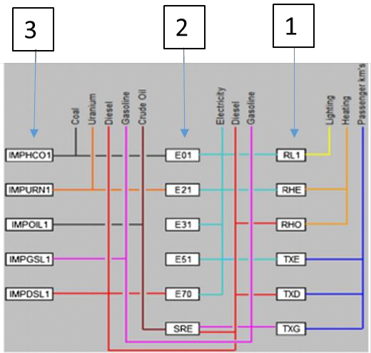
Strategy to add a dummy technology in the RES.
Upperlimit and maxlimit increase
If the optimization has no feasible solution, then one issue might be that certain upper limits or maximum limits have become binding and prevent the solver from finding a feasible solution. There are upper limits defined by the user but also default upper limits on parameters that are embedded in the code for OSeMOSYS (either in terms of Capacity or Activity). To find these “upperlimit” and “maxlimit” search in the code (Ctrl+F) and take a step-by-step approach both in the input file and in the OSeMOSYS code to identify if the issue is in one of these constraints. One option is for example to write a hash “#” before one or several of these constraints, thus commenting them out. If the model then solves successfully, it is clear that these constraints (potentially in combination with others) where the reason for the previous infeasibility and adjustments in the data file are necessary. These could involve correcting incorrectly entered input data or raising the maximum limits defined in the data file. Of course, the commented out constraints would have to be uncommented in the corrected model by removing the hash “#” sign.
Starting the chain with a technology
In OSeMOSYS the chain always needs to start with a technology. This means that in order to have a fuel in the system, a technology needs to be defined as the producer. For instance, in an oil power plant we define oil as an input (parameter “InputActivityRatio”) and electricity as an output (parameter “OutputActivityRatio”). However, the oil has to be produced by another technology, such as “oil import”. In this case the oil import technology has NO input (unless we are defining the entire oil supply chain as well), but only oil as an output. Another example where an error is common is when defining a renewable energy technology, such as solar photovoltaics (PV). For example, in the case of a PV, the output is electricity. You can choose to define sunlight or have no input at all. In the former case though, a technology providing this sunlight needs to be defined also (e.g. “Sun”).
It is advisable to construct a Reference Energy System (similar to the Figure above, under Adding a dummy technology), before starting to construct the model. This will help visualize the overall system with its interconnections and it will facilitate in the quick identification of potential sources of error.
Incorrect demand split definitions
A common mistake is misrepresenting the seasonal/daily variation of demand. To avoid this, make sure that the sum of all timeslices in the parameter “SpecifiedDemandProfile” adds up to 1. An indication that this may be a problem is if the total production of the respective fuel is lower (in case sum of “SpecifiedDemandProfile” specified is lower than 1) or higher (in case the sum of “SpecifiedDemandProfile” specified exceeds 1) than what defined in the parameter “SpecifiedAnnualDemand”.
Setting the correct default values
Each parameter is typically defined with a default value. This in turn is assumed to be the value for all the parameters of technologies, fuels etc. that the modeller chooses not to define explicitly. Make sure to go through all default values and verify that these are not the source of a problem. For instance, one common mistake is setting a default value for the parameter “DiscountRate” at 5 (indicating 500%) instead of 0.05 (indicating 5%). As a result, since OSeMOSYS optimizes the discounted cost of the system, the difference between the various alternative pathways is assumed to be minimal due to the incredibly high discount rate and the resulting optimal solution is simply a random choice from the vast solution space. As a measure of good practice, it is advised that appropriate default values are chosen for all parameters at the very beginning of model development.
Capacity factors
The parameter Capacity Factor in OSeMOSYS represents an upper limit on the capacity of a specific technology that can operate in each time slice. For fossil fuel fired power plants, e.g. steam cycles fuelled by coal, it may be around 85% of the installed capacity, meaning that in a given timeslice at most 85% of the capacity can be used, due to technological constraints. For renewables like PV panels or wind turbines it can be used in a slightly different way (and it usually is): it still represents an upper limit on the ratio of the capacity that can be used, but due to the availability of resources, rather than to technological constraints. For instance, for PV panels at night it is set to 0, so that the user makes sure the model won’t choose to use PV panels when the sun is not there.